Small-world networks

In this blog post I describe some basic terms used in graph theory then talk about the differences between regular and random graphs then conclude with small-world networks. In neuroscience research there have been many ideas about how to model neural connections and how to extract meaningful patterns from data. Graph theory has been used as a basis for understanding these networks.

1. Terminology

Firstly, I would like to start this post with explaining some terminology from graph theory. A graph consists of vertices and edges. Vertices can be described as nodes or points and an edge is a connection between two vertices. An analogy to a graph is a social network where a vertex represents a person and an edge represents a friendship between the two people.

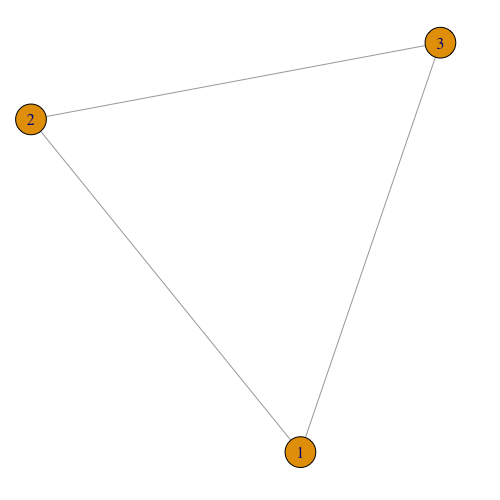
Figure 1

Let us consider a graph with three vertices as depicted in Figure 1. It has the vertex set $V = \{v_{1}, v_{2}, v_{3}\}$. Connecting these vertices are the set of edges $E=\{v_{1}v_{2},v_{1}v_{3},v_{2}v_{3}\}$. An edge is written as $v_iv_j$ representing an undirected connection between $v_i$ and $v_j$. As the graph is undirected, the order of the vertices in an edge do not matter, edge $v_{i}v_{j}$ is the equivalent to $v_{j}v_{i}$.

The degree of a vertex denotes the number of connections it has with other vertices. If a vertex has no connections it has degree $k = 0$. In the graph below each vertex has degree 4 ($k = 4$), i.e. 4 neighbours, and it can also be described as being a 4-regular graph or a quartic graph. The order of the graph is the number of nodes and the size of the graph is the number of edges. So in this example we have order 10 and size 20.

The maximum number of edges in a graph can be calculated by the formula $\frac {n(n-1)}{2}$, $n$ is the number of vertices, for Figure 2 the maximum number of edges is $45$. The path length $d(v_{i},v_{j})$ is the shortest distance between a pair of vertices $v_{i}$ and $v_{j}$, in Figure 2 $d(v_9,v_5) = 2$, whereas $d(v_9,v_8) = 1$. To calculate the average path length or characteristic path length (Watts & Strogatz, 1998) in a connected graph we calculate the average path lengths over all pairs of vertices: $L(G) = \frac {1}{n(n-1)} \sum\limits_{v_{i},v_{j}}d(v_{i},v_{j})$. The average path length of Figure 1 with distances $d(v_{1},v_{2}) = d(v_{1},v_{3}) = d(v_{2},v_{3}) = 1$ is $\frac {1+1+1}{3} = 1$.

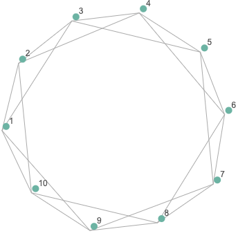
Figure 1

2. Regular & Random Graphs

Graphs have been used to make sense of structures and their connections in nature. The types of networks in many aspects of life were thought to be either regular or random. First of all, what is meant by a regular network? It is very much like the graph in Figure 2 where all nodes have the same number of neighbours (degree). A random graph on the other hand is one which has nodes and edges arranged by a random procedure. The edges in a random graph are assigned by a given probability p. With a probability $p = 0.2$ and a maximum of $n = 45$ edges we might expect to have $pn = 9$ edges in our graph (Erdős & Rényi, 1959). In contrast, when $p = 1$ then every node is connected to every other node in the graph.

3. Small-world networks (Watts & Strogatz 1998)

Based on a concept of ‘six degrees of separation’ that one person is merely six or fewer social connections away from another person, the small-world network model assumes that networks in real-life are not completely random. This was tested by psychologist, Milgram in his famous ‘small-world experiment’ using average path lengths within social networks (Milgram, 1967). In Watts & Strogatz’s paper, they used three different datasets for creating graphs: a film actors’ network, a neural network of the C.elegans worm and an electrical power grid. They found that neither the regular nor the random models were a good fit, but instead the ‘small-world network’ which is a hybrid of the two. Whereby so-called ‘shortcuts’ are added in a ‘random’ way and they act as a way of decreasing the path length between nodes. Probability $p_{rewire}$ (labelled this to differentiate it from probability used above) was used to rewire the connections in a regular ring lattice so when $p_{rewire} = 0$ the lattice stayed the same and when $p_{rewire} = 1$ all of the edges were rewired randomly.

The two measures: characteristic path length and clustering coefficient were used to compare the networks. The clustering coefficient of a vertex $v$ is actual number of edges divided by the maximum number of possible edges. The clustering coefficient of a graph is the degree to which vertices in a graph cluster and calculated as the average clustering coefficient over all vertices. The characteristic path length is the average shortest path length between all pairs of vertices as described in the Terminology section. What makes a small-world network different from regular and random graphs is that the distance between two randomly chosen vertices grows logarithmically to the number of vertices: $L\propto \log N$. Small-world networks are efficient because they have a low characteristic path length and high clustering between vertices.

In summary, the characteristics of each type of graph are as follows:

Regular	Small-world	Random
High path length	Low path length	Low path length
High clustering	High clustering	Low clustering

Small-world networks have been used to explain biological mechanisms and I will talk about how they has been used in neuroscience research in my next blog post.

References

Erdős, P., & Rényi, A. (1959). On random graphs I. Publ. math. debrecen, 6(290-297), 18.

Milgram, S. (1967). The small world problem. Psychology today, 2(1), 60-67.

Watts, D. J., & Strogatz, S. H. (1998). Collective dynamics of ‘small-world’ networks. Nature, 393(6684), 440-442.