OASIS Dataset Analysis (II)
Link to the original paper https://www.ncbi.nlm.nih.gov/pmc/articles/PMC2895005/
Aim of this post: use linear mixed-effects models to look at the fixed and random effects in this dataset.
Linear mixed-effects models (LME)
Linear mixed effects models are based on the simple linear regression model that allow for the measure of both fixed and random effects. Definitions of random and fixed effects are not necessarily to do with the variables themselves but vary depending on the research question. Fixed effects are the effects of variables of interest. In this blog for example one of the variables of interest is the MMSE score so we want to look at its effect on the likelihood of the subject developing dementia. Whereas random effects are usually any variation are a result of regions that are not of interest to us. For example variability between subjects can be seen as a random effect. These models are used for when there is non-independence in the data and are also good for designs with repeated measures as well as data with missing values. Whereas with an ANOVA test, independence of variables and a normally distributed sample is assumed.
Loading and Preprocessing
import pandas as pd
oasis_df = pd.read_csv('oasis_longitudinal.csv')

oasis_df = oasis_df.drop(['MRI ID','MR Delay', 'Hand'], axis=1)
oasis_df = oasis_df.rename({'Subject ID': 'Subject_ID', "M/F" : 'Gender'}, axis=1)
oasis_df['Gender'] = oasis_df['Gender'].astype('category')
oasis_df['Gender'] = oasis_df['Gender'].cat.codes

oasis_df
| Subject_ID | Group | Visit | Gender | Age | EDUC | SES | MMSE | CDR | eTIV | nWBV | ASF | |
|---|---|---|---|---|---|---|---|---|---|---|---|---|
| 0 | OAS2_0001 | Nondemented | 1 | 1 | 87 | 14 | 2.0 | 27.0 | 0.0 | 1987 | 0.696 | 0.883 |
| 1 | OAS2_0001 | Nondemented | 2 | 1 | 88 | 14 | 2.0 | 30.0 | 0.0 | 2004 | 0.681 | 0.876 |
| 2 | OAS2_0002 | Demented | 1 | 1 | 75 | 12 | NaN | 23.0 | 0.5 | 1678 | 0.736 | 1.046 |
| 3 | OAS2_0002 | Demented | 2 | 1 | 76 | 12 | NaN | 28.0 | 0.5 | 1738 | 0.713 | 1.010 |
| 4 | OAS2_0002 | Demented | 3 | 1 | 80 | 12 | NaN | 22.0 | 0.5 | 1698 | 0.701 | 1.034 |
| ... | ... | ... | ... | ... | ... | ... | ... | ... | ... | ... | ... | ... |
| 368 | OAS2_0185 | Demented | 2 | 1 | 82 | 16 | 1.0 | 28.0 | 0.5 | 1693 | 0.694 | 1.037 |
| 369 | OAS2_0185 | Demented | 3 | 1 | 86 | 16 | 1.0 | 26.0 | 0.5 | 1688 | 0.675 | 1.040 |
| 370 | OAS2_0186 | Nondemented | 1 | 0 | 61 | 13 | 2.0 | 30.0 | 0.0 | 1319 | 0.801 | 1.331 |
| 371 | OAS2_0186 | Nondemented | 2 | 0 | 63 | 13 | 2.0 | 30.0 | 0.0 | 1327 | 0.796 | 1.323 |
| 372 | OAS2_0186 | Nondemented | 3 | 0 | 65 | 13 | 2.0 | 30.0 | 0.0 | 1333 | 0.801 | 1.317 |
373 rows × 12 columns
The dummy coding is done here for the ‘Group’ column as these are categorical. Also we want to remove the participants who already have dementia as we want to see what potentially affects whether someone develops dementia.
one_visit = oasis_df[oasis_df['Visit'] == 1] # subset of data
dummies = pd.get_dummies(one_visit["Group"]) # dummy coding for group
one_visit = one_visit.merge(dummies, left_index=True, right_index=True).dropna()
one_visit = one_visit[ one_visit["Demented"] != 1 ] # removed participants who already have dementia
one_visit.head()
| Subject_ID | Group | Visit | Gender | Age | EDUC | SES | MMSE | CDR | eTIV | nWBV | ASF | Converted | Demented | Nondemented | |
|---|---|---|---|---|---|---|---|---|---|---|---|---|---|---|---|
| 0 | OAS2_0001 | Nondemented | 1 | 1 | 87 | 14 | 2.0 | 27.0 | 0.0 | 1987 | 0.696 | 0.883 | 0 | 0 | 1 |
| 5 | OAS2_0004 | Nondemented | 1 | 0 | 88 | 18 | 3.0 | 28.0 | 0.0 | 1215 | 0.710 | 1.444 | 0 | 0 | 1 |
| 7 | OAS2_0005 | Nondemented | 1 | 1 | 80 | 12 | 4.0 | 28.0 | 0.0 | 1689 | 0.712 | 1.039 | 0 | 0 | 1 |
| 13 | OAS2_0008 | Nondemented | 1 | 0 | 93 | 14 | 2.0 | 30.0 | 0.0 | 1272 | 0.698 | 1.380 | 0 | 0 | 1 |
| 19 | OAS2_0012 | Nondemented | 1 | 0 | 78 | 16 | 2.0 | 29.0 | 0.0 | 1333 | 0.748 | 1.316 | 0 | 0 | 1 |
Questions
- Which factors most affect whether a participant develops dementia?
- Which factors affect participants’ scores from baseline compared to their second visit?
For this post, linear mixed effects models are used instead.
both_visits = oasis_df[oasis_df['Visit'] <= 2].dropna()

both_visits = both_visits.groupby('Subject_ID').filter(lambda x: len(x) == 2)
both_visits_EDUC_SES_gender = both_visits[['Subject_ID','EDUC','SES','Gender']] #keep values that do not change
both_visits = both_visits.sort_values(["Subject_ID", "Visit"])
both_visits_diff = both_visits.groupby(['Subject_ID'])[['Age', 'MMSE',
                                                        'CDR', 'eTIV', 'nWBV', 'ASF']].diff().dropna()
both_visits = both_visits[["Subject_ID", "Group"]].merge(both_visits_diff, left_index=True, right_index=True)
both_visits = both_visits.merge(both_visits_EDUC_SES_gender, left_index=True, right_index=True, suffixes=(None,'_y'))
both_visits = both_visits.drop(columns = ['Subject_ID_y'])

dummies = pd.get_dummies(both_visits["Group"])
both_visits = both_visits.merge(dummies, left_index=True, right_index=True).dropna()

both_visits = both_visits[both_visits["Demented"] != 1]
both_visits = both_visits.drop(columns='Group')
Preliminary Tests
import numpy as np
import statsmodels.formula.api as smf
import statsmodels.api as sm
import pylab as py
import seaborn as sns
import matplotlib.pyplot as plt
both_visits.head()
| Subject_ID | Age | MMSE | CDR | eTIV | nWBV | ASF | EDUC | SES | Gender | Converted | Demented | Nondemented | |
|---|---|---|---|---|---|---|---|---|---|---|---|---|---|
| 1 | OAS2_0001 | 1.0 | 3.0 | 0.0 | 17.0 | -0.015 | -0.007 | 14 | 2.0 | 1 | 0 | 0 | 1 |
| 6 | OAS2_0004 | 2.0 | -1.0 | 0.0 | -15.0 | 0.008 | 0.018 | 18 | 3.0 | 0 | 0 | 0 | 1 |
| 8 | OAS2_0005 | 3.0 | 1.0 | 0.5 | 12.0 | -0.001 | -0.007 | 12 | 4.0 | 1 | 0 | 0 | 1 |
| 14 | OAS2_0008 | 2.0 | -1.0 | 0.0 | -15.0 | 0.005 | 0.016 | 14 | 2.0 | 0 | 0 | 0 | 1 |
| 20 | OAS2_0012 | 2.0 | 0.0 | 0.0 | -10.0 | -0.010 | 0.010 | 16 | 2.0 | 0 | 0 | 0 | 1 |
model_fit = smf.ols('Converted ~ Age+EDUC+SES+MMSE+eTIV+nWBV+ASF+Gender', data=both_visits).fit()

X = pd.DataFrame(both_visits, columns=['Age','EDUC','SES', 'MMSE','eTIV','nWBV','ASF', 'Gender'])
y = pd.DataFrame(both_visits.Converted)
dataframe = pd.concat([X, y], axis=1)

table = sm.stats.anova_lm(model_fit, typ=2)
with pd.option_context('display.max_rows', None, 'display.max_columns', None):
    display(table.sort_values("F", ascending=False))
| sum_sq | df | F | PR(>F) | |
|---|---|---|---|---|
| MMSE | 1.274274 | 1.0 | 12.471175 | 0.000720 |
| SES | 0.962042 | 1.0 | 9.415391 | 0.003019 |
| Age | 0.602529 | 1.0 | 5.896878 | 0.017632 |
| EDUC | 0.545404 | 1.0 | 5.337811 | 0.023696 |
| Gender | 0.136944 | 1.0 | 1.340251 | 0.250764 |
| ASF | 0.035178 | 1.0 | 0.344279 | 0.559180 |
| eTIV | 0.033727 | 1.0 | 0.330083 | 0.567377 |
| nWBV | 0.000235 | 1.0 | 0.002301 | 0.961871 |
| Residual | 7.458961 | 73.0 | NaN | NaN |
#model values
model_fitted_y = model_fit.fittedvalues
model_residuals = model_fit.resid
model_norm_residuals = model_fit.get_influence().resid_studentized_internal
model_norm_residuals_abs_sqrt = np.sqrt(np.abs(model_norm_residuals))
model_abs_resid = np.abs(model_residuals)
model_leverage = model_fit.get_influence().hat_matrix_diag
model_cooks = model_fit.get_influence().cooks_distance[0]
Q-Q plot
In order to check whether the data used is normally distributed, we can use a quantile-quantile plot. It is a probability plot comparing two probability distributions where the x coordinate is a theoretical quantile and the y-coordinate is the quantile from the actual data. If the distribution is normal then the points will roughly lie on the line y = x.
from statsmodels.graphics.gofplots import ProbPlot

QQ = ProbPlot(model_norm_residuals)
plot_lm_2 = QQ.qqplot(line='45', alpha=0.5, color='#4C72B0', lw=1)
plot_lm_2.axes[0].set_title('Normal Q-Q Plot')
plot_lm_2.axes[0].set_xlabel('Theoretical Quantiles')
plot_lm_2.axes[0].set_ylabel('Standardized Residuals');
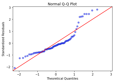
The Q-Q plot shows that there are many outliers that do not fit well on the line indication a deviation from a normal distribution. This makes it evident that another type of statistical model might be better for this dataset.
Shapiro-Wilk Test
Another more robust test for normality is the Shapiro-Wilk Test (Shapiro & Wilk, 1965) and this was applied to the measures from the data below. For this test the null hypothesis if that the observations are normally distributed.
from scipy.stats import shapiro
from tabulate import tabulate
shapiro_results = []

for column in both_visits:
    try:
        s = shapiro(both_visits[column])
        shapiro_results.append([column, s.statistic, s.pvalue])
    except Exception as e:
        pass

df = pd.DataFrame(shapiro_results)
df = df.drop([9,10,11], axis=0) #drop dummy measures
print('Shapiro-Wilk Test \n')
print(tabulate(df, headers=['Measure', 'W statistic', 'p value'],showindex="never",tablefmt="presto"))
Shapiro-Wilk Test

 Measure   |   W statistic |     p value
-----------+---------------+-------------
 Age       |      0.84819  | 1.06861e-07
 MMSE      |      0.857197 | 2.17703e-07
 CDR       |      0.431455 | 3.12775e-16
 eTIV      |      0.859982 | 2.72737e-07
 nWBV      |      0.987887 | 0.640755
 ASF       |      0.878246 | 1.28239e-06
 EDUC      |      0.933238 | 0.000356511
 SES       |      0.876038 | 1.05635e-06
 Gender    |      0.578552 | 5.53986e-14


/usr/local/lib/python3.8/site-packages/scipy/stats/morestats.py:1678: UserWarning: Input data for shapiro has range zero. The results may not be accurate.
  warnings.warn("Input data for shapiro has range zero. The results "
The only variable that seems to be normally distributed here is the nWBV with W = 0.99 and p value = .64, indicating normality. This is expected as these values have already been normalised as mentioned in the paper.
Linear Mixed Effects Models
In this first model, using the statsmodel function mixedlm(), five of the variables are treated as fixed effects with subject as the random effect as defined in the argument groups. This would be the equivalent of Converted ~ MMSE… + (1 | Subject) in R. All of the effects are calculated here in terms of interactions and simple effects. By default and because I have not specified it there is a random intercept for each group. The Bayesian Information Criteria (BIC) is pulled here as well to have a criteria for model fitting: the higher the score, the better. However it should be noted that every time a variable is added this score will increase.
#fit model
mixed = smf.mixedlm('Converted ~ MMSE*nWBV*eTIV*EDUC*SES',data=both_visits, groups=both_visits['Subject_ID'])
mixed_fit = mixed.fit(reml=False)
/usr/local/lib/python3.8/site-packages/statsmodels/regression/mixed_linear_model.py:2189: ConvergenceWarning: The Hessian matrix at the estimated parameter values is not positive definite.
  warnings.warn(msg, ConvergenceWarning)
#print summary
mixed_fit_results = mixed_fit.summary()
print(mixed_fit_results)
BIC_1 = mixed_fit.bic
print('Bayesian Information Criteria (BIC): ', BIC_1)
                Mixed Linear Model Regression Results
======================================================================
Model:                 MixedLM      Dependent Variable:      Converted
No. Observations:      82           Method:                  ML
No. Groups:            82           Scale:                   0.0307
Min. group size:       1            Log-Likelihood:          -1.9069
Max. group size:       1            Converged:               Yes
Mean group size:       1.0
----------------------------------------------------------------------
                         Coef.  Std.Err.   z    P>|z|  [0.025   0.975]
----------------------------------------------------------------------
Intercept                 0.094    0.715  0.131 0.896   -1.308   1.496
MMSE                     -0.904    0.732 -1.234 0.217   -2.338   0.531
nWBV                    -21.038   77.849 -0.270 0.787 -173.618 131.543
MMSE:nWBV               -43.271   60.534 -0.715 0.475 -161.916  75.374
eTIV                      0.007    0.050  0.132 0.895   -0.092   0.106
MMSE:eTIV                 0.252    0.075  3.379 0.001    0.106   0.398
nWBV:eTIV                -2.221    6.510 -0.341 0.733  -14.980  10.538
MMSE:nWBV:eTIV           17.493    5.061  3.456 0.001    7.573  27.413
EDUC                      0.006    0.043  0.149 0.881   -0.078   0.091
MMSE:EDUC                 0.078    0.050  1.552 0.121   -0.021   0.177
nWBV:EDUC                 1.439    5.041  0.285 0.775   -8.442  11.319
MMSE:nWBV:EDUC            5.166    4.077  1.267 0.205   -2.825  13.156
eTIV:EDUC                -0.000    0.003 -0.003 0.998   -0.006   0.006
MMSE:eTIV:EDUC           -0.016    0.005 -3.350 0.001   -0.026  -0.007
nWBV:eTIV:EDUC            0.013    0.409  0.032 0.974   -0.788   0.814
MMSE:nWBV:eTIV:EDUC      -1.143    0.328 -3.485 0.000   -1.786  -0.500
SES                       0.242    0.252  0.959 0.337   -0.253   0.737
MMSE:SES                  0.267    0.251  1.061 0.289   -0.226   0.760
nWBV:SES                 34.571   27.602  1.252 0.210  -19.528  88.671
MMSE:nWBV:SES            27.258   24.879  1.096 0.273  -21.503  76.020
eTIV:SES                  0.021    0.022  0.960 0.337   -0.022   0.065
MMSE:eTIV:SES            -0.103    0.029 -3.577 0.000   -0.159  -0.046
nWBV:eTIV:SES             0.131    2.114  0.062 0.950   -4.011   4.274
MMSE:nWBV:eTIV:SES       -7.349    1.830 -4.015 0.000  -10.936  -3.761
EDUC:SES                 -0.021    0.018 -1.156 0.248   -0.055   0.014
MMSE:EDUC:SES            -0.026    0.019 -1.368 0.171   -0.063   0.011
nWBV:EDUC:SES            -2.718    2.036 -1.335 0.182   -6.708   1.271
MMSE:nWBV:EDUC:SES       -2.800    1.827 -1.533 0.125   -6.381   0.781
eTIV:EDUC:SES            -0.001    0.002 -0.892 0.372   -0.004   0.002
MMSE:eTIV:EDUC:SES        0.007    0.002  3.341 0.001    0.003   0.011
nWBV:eTIV:EDUC:SES        0.069    0.144  0.479 0.632   -0.214   0.352
MMSE:nWBV:eTIV:EDUC:SES   0.493    0.135  3.656 0.000    0.229   0.758
Group Var                 0.031
======================================================================

Bayesian Information Criteria (BIC):  153.6421986502787
#convert summary results to dataframe
def summary_to_df(results):
    pvals = results.pvalues
    coeff = results.params
    conf_lower = results.conf_int()[0] #lower confidence interval of the fitted parameters
    conf_higher = results.conf_int()[1]

    results_df = pd.DataFrame({"pvals":pvals,
                               "coeff":coeff,
                               "conf_lower":conf_lower,
                               "conf_higher":conf_higher
                                })

    results_df = results_df[["coeff","pvals","conf_lower","conf_higher"]]
    return results_df
summary_df = summary_to_df(mixed_fit)
sig_pvals = summary_df[summary_df ['pvals']<= 0.05]
sig_pvals
| coeff | pvals | conf_lower | conf_higher | |
|---|---|---|---|---|
| MMSE:eTIV | 0.251948 | 0.000726 | 0.105827 | 0.398068 |
| MMSE:nWBV:eTIV | 17.493033 | 0.000548 | 7.572879 | 27.413187 |
| MMSE:eTIV:EDUC | -0.016371 | 0.000809 | -0.025949 | -0.006792 |
| MMSE:nWBV:eTIV:EDUC | -1.143294 | 0.000492 | -1.786245 | -0.500342 |
| MMSE:eTIV:SES | -0.102714 | 0.000348 | -0.158998 | -0.046431 |
| MMSE:nWBV:eTIV:SES | -7.348724 | 0.000059 | -10.936178 | -3.761270 |
| MMSE:eTIV:EDUC:SES | 0.006792 | 0.000834 | 0.002808 | 0.010776 |
| MMSE:nWBV:eTIV:EDUC:SES | 0.493338 | 0.000256 | 0.228863 | 0.757812 |
We can see the significant effects of the interactions here. It seems that the combinations of these variables is an important measure for the question.
#fit model 2
mixed2 = smf.mixedlm('Converted ~ MMSE+SES+EDUC+nWBV+eTIV+Age+Gender',data=both_visits, groups=both_visits['Subject_ID'])
mixed2_fit = mixed2.fit(reml=False)

print(mixed2_fit.summary())
print('Bayesian Information Criteria (BIC): ', mixed2_fit.bic)
         Mixed Linear Model Regression Results
=======================================================
Model:            MixedLM Dependent Variable: Converted
No. Observations: 82      Method:             ML
No. Groups:       82      Scale:              0.0457
Min. group size:  1       Log-Likelihood:     -18.2564
Max. group size:  1       Converged:          Yes
Mean group size:  1.0
-------------------------------------------------------
             Coef.  Std.Err.   z    P>|z| [0.025 0.975]
-------------------------------------------------------
Intercept     0.849    0.199  4.274 0.000  0.460  1.239
MMSE         -0.098    0.026 -3.792 0.000 -0.149 -0.048
SES          -0.144    0.029 -4.997 0.000 -0.200 -0.087
EDUC         -0.043    0.009 -4.695 0.000 -0.061 -0.025
nWBV         -0.553    4.346 -0.127 0.899 -9.071  7.966
eTIV         -0.000    0.002 -0.021 0.983 -0.003  0.003
Age           0.109    0.041  2.636 0.008  0.028  0.189
Gender        0.089    0.074  1.205 0.228 -0.056  0.233
Group Var     0.046
=======================================================

Bayesian Information Criteria (BIC):  80.58007408355029


/usr/local/lib/python3.8/site-packages/statsmodels/regression/mixed_linear_model.py:2189: ConvergenceWarning: The Hessian matrix at the estimated parameter values is not positive definite.
  warnings.warn(msg, ConvergenceWarning)
The second LME model only measures the simple effects of the fixed effects. The BIC is a lot smaller as there are fewer observations.
summary_df2 = summary_to_df(mixed2_fit)
sig_pvals2 = summary_df2[summary_df2['pvals'] <= 0.05]
sig_pvals2
| coeff | pvals | conf_lower | conf_higher | |
|---|---|---|---|---|
| Intercept | 0.849244 | 1.921953e-05 | 0.459778 | 1.238711 |
| MMSE | -0.098328 | 1.494001e-04 | -0.149149 | -0.047506 |
| SES | -0.143899 | 5.828538e-07 | -0.200342 | -0.087456 |
| EDUC | -0.042990 | 2.666300e-06 | -0.060937 | -0.025043 |
| Age | 0.108547 | 8.391635e-03 | 0.027835 | 0.189259 |
The estimated p values show that the four variables that seem to have the most effect on the Converted variable is: MMSE, SES, EDUC and Age. Age is perhaps a variable that should not be included in the model as dementia is an age-related disorder we would expect that as age increases so does the risk of dementia. However it is interesting to see SES, MMSE and EDUC which are most likely connected especially in certain countries with starker disparities in wealth. Let’s go back to the original dataset and look at these potential relationships. I have used a subset of the dataset named one_visit which contains only the first visit i.e. the baseline values because all of the participants had at least one visit. Also the effect of time on the scores especially for MMSE will change and there will be multiple scores for one participant.
oasis_df2 = oasis_df.dropna() #remove missing scores
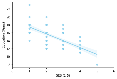
g = sns.regplot(x='SES',y='EDUC', data=one_visit,color="skyblue", scatter_kws={'s':30}, label = 'A');
g = g.set(xlim=(0,6), xlabel="SES (1-5)", ylabel="Education (Years)")
correlation_matrix = np.corrcoef(one_visit['SES'], one_visit['EDUC'])
correlation_xy = correlation_matrix[0,1]
r_squared = correlation_xy**2
print("R-Squared:","{:.2f}".format(r_squared))
R-Squared: 0.47
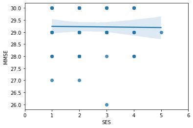
g2 = sns.regplot(x='SES',y='MMSE', data=one_visit);
g2 = g2.set(xlim=(0, 6))

correlation_matrix = np.corrcoef(one_visit['SES'], one_visit['MMSE'])
correlation_xy = correlation_matrix[0,1]
r_squared = correlation_xy**2

print("R-Squared:","{:.4f}".format(r_squared))
R-Squared: 0.0002
g3 = sns.regplot(x='EDUC',y='MMSE', data=one_visit, color="g");
g3 = g3.set(xlim=(7, 25))

oasis_df2 = one_visit.dropna()
correlation_matrix = np.corrcoef(one_visit['EDUC'], one_visit['MMSE'])
correlation_xy = correlation_matrix[0,1]
r_squared = correlation_xy**2

print("R-Squared:","{:.2f}".format(r_squared))
R-Squared: 0.01
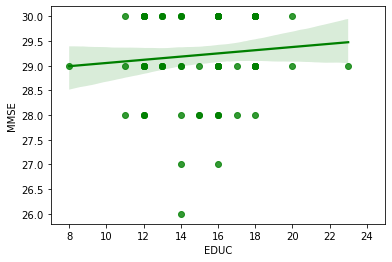
Running the simple linear regression models comparing two of the variables at a time, it is evident that in this dataset EDUC, MMSE & SES do not correlate that well with R-squared values of 0.47, 0.0002 & 0.01. Although Education and SES seem to show a pattern in the graph it is not a strong enough correlation to assume a connection between the two.
LME models are common practice in longitudinal studies and did give more insight into the data compared to the ANOVA which is probably not the best method to use for this dataset due to missing data and non-independence of variables. In addition, the models that I used may not be the best for this dataset either and can be interpreted in other ways for example some might suggest that socioeconomic status could be treated as a random effect depending on how the sample was collected. Another aspect I did not delve into is possible nested effects.
References
Shapiro, S. S., & Wilk, M. B. (1965). An analysis of variance test for normality (complete samples). Biometrika, 52(3/4), 591-611.