Clustering

The word cluster varies across different fields, but ultimately has the same meaning of the close positioning of objects/living things that are similar to each other. In machine learning, clustering is an unsupervised method with the aim of grouping the data into clusters. The aim is to have observations that have more common traits than with other groups. Clustering can be performed in many ways: k-means, hierarchical clustering, Gaussian mixture modelling, just to name a few. In this post, the focus will be on hierarchical clustering as it has been the method I have been using the past few months. Hierarchical clustering outputs a structure called a dendrogram that explains visually how the clusters are separated.

Use cases

These use cases are from a chapter on clustering (Gore, 2000).

• Grouping based on multivariate similarity
• Data exploration
• Develop a classification system
• Finding latent connections in the data
• Use for confirmation of previous hypotheses or findings

Bottom-up vs Top-down

There are two main clustering approaches: bottom-up & top-down. The bottom-up approach refers to each data point starting as an individual cluster which are then paired and move up the series of trees. This type of clustering is also called ‘agglomerative hierarchical clustering’ because of the sequential merging of these single clusters. In the top-down approach, the data points are all together in one cluster and move down the hierarchy splitting from each other in a recursive manner.

Steps in a nutshell

Let’s assume that you have a somewhat ‘clean’ dataset with preprocessing all done and you are ready to start your analysis. Also make sure that any scaling of the data is done before running the clustering.

1. Choose features to use for clustering
2. Calculate similarity/dissimilarity (distance)
   Regardless of which method you choose, we need to calculate the similarity of the data points
3. A linkage criterion is then used to determine the pairwise distances of the data points
4. Choose optimal k (number of clusters)

Example

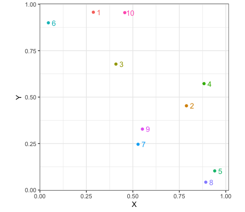
For our example, we are not really using any features, but for datasets that actually have some meaning these might be variables that are thought of as having an importance for understanding the data. We could have groups of patients with different diseases and our features could be results from various medical tests like blood pressure. Using a randomly generated set of x and y coordinates for our example dataset in R , we can look at the steps of this method. Agglomerative clustering and average linkage is used in this blog. The scatterplot below shows our data points in relation to each other. It is already evident, which points would be clustered together like datapoints $9$ & $7$.

The next step is to calculate a distance matrix so we can compare how close are data points are to each other. For this example, Euclidean distance is used, but there are many other distance measures you can use and this varies depending on your dataset. The distance between two points is calculated using Pythagorean theorem. Considering we have two points in a 2D space, $a$ with coordinates $(a_1,a_2)$ and $b$ with $(b_1,b_2)$, the distance between the two would be: $d(a,b) = \sqrt{ (a_1 - b_1)^2 + (a_2-b_2)^2}$
You can simply use the dist() function in R, but I have also done this manually for demonstration purposes.

#calculate distance matrix
#manual way

dist_matrix <- matrix(nrow=10, ncol=10)
for (i in 1:10){
  for (j in 1:10){
    if (i > j){
      dist_val <- sqrt((clust_data$X[i] - clust_data$X[j])**2 + (clust_data$Y[i] - clust_data$Y[j])**2)
      dist_matrix[i,j] <- dist_val
    }
  }
}

#dist() function
dist_matrix_2 <- dist(clust_data, method="euclidean",diag=F)

The distance matrix should have the same number of rows and columns i.e the number of datapoints. Here, we only have 10 so this would be a 10x10 matrix with the pairwise distances.

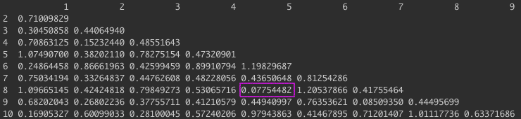
The next step involves calculating the distance between clusters and merging them together. We first start by finding the smallest distance between two points to make a cluster and update the values in our distance matrix. For this example, the average distance between clusters is used (average linkage). Again, you can use the hclust() function or you can do this by hand. I have written a function for this linkage below. In our distance matrix (above), we can see that the smallest distance is between point $5$ & $8$. So now we can merge these two points and compare the distance between this cluster with the other points in our matrix. To do this we take the average distance between points, for the first data point we would calculate: $d((5,8),1) = \frac{d(5,1) + d(8,1)}{2}$

#average linkage function
average_linkage <- function(mat, datapoint) {
  min_dist <- min(mat, na.rm = TRUE) #find smallest distance value
  min_index <- which(mat==min_dist, arr.ind=TRUE)[1,] #get row and col indices
  min_row <- index[["row"]]
  min_col <- index[["col"]]
  comp_pair_1 <- if(is.na((mat[min_row,datapoint]))) {(mat[datapoint, min_row])} else {mat[min_row,datapoint]}
  comp_pair_2 <- if(is.na((mat[min_col,datapoint]))) {(mat[datapoint, min_col])} else {mat[min_col,datapoint]}
  new_val <- (comp_pair_1  + comp_pair_2) / 2 #calculate average linkage
  cluster_name <- c(paste0(min_row, "_", min_col))
  return(c(cluster_name, new_val))
}

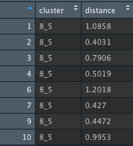
This are the new distance values comparing our first cluster, named 8_5 with the other points in our dataset. This step is repeated until there is only one distance value left, in other words, when we only have one cluster left containing all of our points.

#hclust() method
tree <- hclust(as.dist(dist_matrix), method = "average")
dend_plot <- as.dendrogram(tree)
plot(dend_plot)
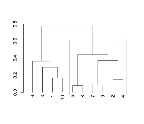
rect.hclust(tree, k = 2, border=color_blind_palette[1:2]) # draw rectangles

By using hclust() this steps are done craftfully in the background making it extremely easy to run clustering even as a beginner. The output from tree, helps us to understand what is happening here.

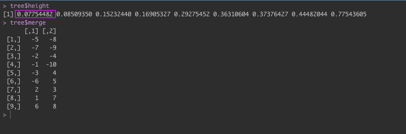
We can see in our tree variable that in height the distance values are increasing in order. The first value is the distance for our first cluster 8_5. Under merge, the negative values represent the individual data points e.g. -5 and -8. Whereas the positive values are the clusters, so in the fifth row we have the two values: -3 and 4 which translates to datapoint 3 & cluster 4 in the row above (1,10). If we look at our dendrogram, 3 is connected to the 1_10 cluster.

As mentioned in the beginning of the blog, the output of this method can be displayed as a dendrogram. I have split this diagram into two clusters just by visually assessing where I think the split makes the most sense. However, there are more scientific ways of choosing the number of clusters ($k$).

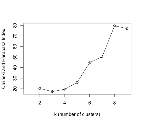
One way of choosing $k$ is to use a cluster validation index for example the Calinski-Harabasz (CH) Index. By measuring the similarity of datapoints to their own cluster (intra-cluster cohesion) in comparison to those in other clusters (inter-cluster separation), a ratio of the two is calculated. The higher this index is, the better the value of k explains the data.
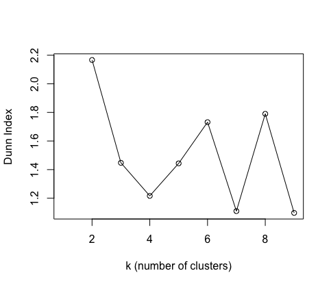
Another validity measure is the Dunn’s Index which similarly to the CH index asseses whether clusters contain points that are close together and those in other clusters are separated. A higher Dunn Index value means better clustering. I have plotted these two indices for number of clusters, but they are not so informative as we only have 10 data points! If one uses a larger dataset, these indices can be helpful at seeing how many cuts to make in the dendrogram. Once you have chosen $k$ you can use the cutree() function

Final comments

How does one know whether the patterns they are seeing have any meaning? Ground-truth labels are not used in clustering, which makes it potentially difficult to be sure that the found clusters make sense to us. This is the beauty and the danger of using clustering. The method can help us find interesting characteristics and connections that we may not have envisioned before running our analyses.

References

Gore, P. A., Jr. (2000). Cluster analysis. In H. E. A. Tinsley & S. D. Brown (Eds.), Handbook of applied multivariate statistics and mathematical modeling (p. 297–321). Academic Press. https://doi.org/10.1016/B978-012691360-6/50012-4